Introduction to Units
ldc relies on the units package to facilitate unit conversions and tracking of units across variables. This is handy if we want to transform units on the fly. I suggest briefly reviewing the units package documentation to become familiar with how units objects are handled. A brief example is shown below:
library(units)
#> udunits database from /usr/share/xml/udunits/udunits2.xml
## generate random data
x <- rlnorm(n = 100, meanlog = log(100), sdlog = log(10))

## attach units, cubic feet per second
x <- set_units(x, "ft^3/s")
x
#> Units: [ft^3/s]
#>   [1]   198.244738     1.377296    22.986791  1744.141817    10.722960
#>   [6]   184.201175     7.096251    82.587769    58.993986   501.604566
#>  [11]    30.155371     6.533947    62.429439 17006.730933  2271.703151
#>  [16]    13.365492   212.617723    27.044502     4.665912    31.864053
#>  [21]    65.564056   528.648919     4.462644  6016.813560     6.588087
#>  [26]    14.502402  1392.888883    45.628694    24.164122    50.279935
#>  [31]    12.234267    44.576009     4.470887    57.691876    40.937223
#>  [36]    44.090073     5.232488   654.161344    28.645744     5.502458
#>  [41]  3303.771576   242.737185    11.105492  1083.307517   853.245838
#>  [46]   110.781533    16.398656   461.277497    69.405736   117.954362
#>  [51]     2.189945   118.595715  3835.141619    30.486449   159.909549
#>  [56]    16.240850   151.832580  1233.088694    54.726964    23.100766
#>  [61]   440.834235   630.081457  1990.296104    12.925787  1587.621005
#>  [66]     6.142746   630.916843 11173.262114    68.351378 13789.569070
#>  [71]     1.573709    32.497518   522.000903    14.542676    54.479840
#>  [76]    31.692962   214.984260    44.418574   114.634036   536.240390
#>  [81]   291.390345    37.438940    94.015468   790.385016  1454.434591
#>  [86]   381.905914    30.497195    37.086893     4.214432   926.021152
#>  [91]  2278.752823    14.901414  2412.694040    34.534378    30.528571
#>  [96]     3.633051  1329.385884   902.954793    87.276794     6.329255
x is a object of type units which can be used with most R expressions:
x * 86400
#> Units: [ft^3/s]
#>   [1]   17128345.4     118998.3    1986058.7  150693853.0     926463.8
#>   [6]   15914981.5     613116.1    7135583.2    5097080.4   43338634.5
#>  [11]    2605424.0     564533.1    5393903.5 1469381552.6  196275152.2
#>  [16]    1154778.5   18370171.3    2336644.9     403134.8    2753054.2
#>  [21]    5664734.5   45675266.6     385572.4  519852691.6     569210.7
#>  [26]    1253007.5  120345599.4    3942319.2    2087780.1    4344186.4
#>  [31]    1057040.6    3851367.1     386284.6    4984578.1    3536976.1
#>  [36]    3809382.3     452087.0   56519540.1    2474992.3     475412.4
#>  [41]  285445864.1   20972492.8     959514.5   93597769.4   73720440.4
#>  [46]    9571524.5    1416843.9   39854375.8    5996655.6   10191256.8
#>  [51]     189211.2   10246669.8  331356235.9    2634029.2   13816185.0
#>  [56]    1403209.4   13118335.0  106538863.1    4728409.7    1995906.2
#>  [61]   38088077.9   54439037.9  171961583.4    1116788.0  137170454.8
#>  [66]     530733.3   54511215.3  965369846.7    5905559.0 1191418767.6
#>  [71]     135968.5    2807785.5   45100878.0    1256487.2    4707058.2
#>  [76]    2738271.9   18574640.1    3837764.8    9904380.7   46331169.7
#>  [81]   25176125.8    3234724.4    8122936.4   68289265.4  125663148.6
#>  [86]   32996670.9    2634957.6    3204307.6     364126.9   80008227.6
#>  [91]  196884243.9    1287482.2  208456765.0    2983770.3    2637668.6
#>  [96]     313895.6  114858940.3   78015294.2    7540715.0     546847.6
The units can be converted:
## convert to cubic feet per day
x <- set_units(x, "ft^3/d")
x
#> Units: [ft^3/d]
#>   [1]   17128345.4     118998.3    1986058.7  150693853.0     926463.8
#>   [6]   15914981.5     613116.1    7135583.2    5097080.4   43338634.5
#>  [11]    2605424.0     564533.1    5393903.5 1469381552.6  196275152.2
#>  [16]    1154778.5   18370171.3    2336644.9     403134.8    2753054.2
#>  [21]    5664734.5   45675266.6     385572.4  519852691.6     569210.7
#>  [26]    1253007.5  120345599.4    3942319.2    2087780.1    4344186.4
#>  [31]    1057040.6    3851367.1     386284.6    4984578.1    3536976.1
#>  [36]    3809382.3     452087.0   56519540.1    2474992.3     475412.4
#>  [41]  285445864.1   20972492.8     959514.5   93597769.4   73720440.4
#>  [46]    9571524.5    1416843.9   39854375.8    5996655.6   10191256.8
#>  [51]     189211.2   10246669.8  331356235.9    2634029.2   13816185.0
#>  [56]    1403209.4   13118335.0  106538863.1    4728409.7    1995906.2
#>  [61]   38088077.9   54439037.9  171961583.4    1116788.0  137170454.8
#>  [66]     530733.3   54511215.3  965369846.7    5905559.0 1191418767.6
#>  [71]     135968.5    2807785.5   45100878.0    1256487.2    4707058.2
#>  [76]    2738271.9   18574640.1    3837764.8    9904380.7   46331169.7
#>  [81]   25176125.8    3234724.4    8122936.4   68289265.4  125663148.6
#>  [86]   32996670.9    2634957.6    3204307.6     364126.9   80008227.6
#>  [91]  196884243.9    1287482.2  208456765.0    2983770.3    2637668.6
#>  [96]     313895.6  114858940.3   78015294.2    7540715.0     546847.6
Units can be plotted:
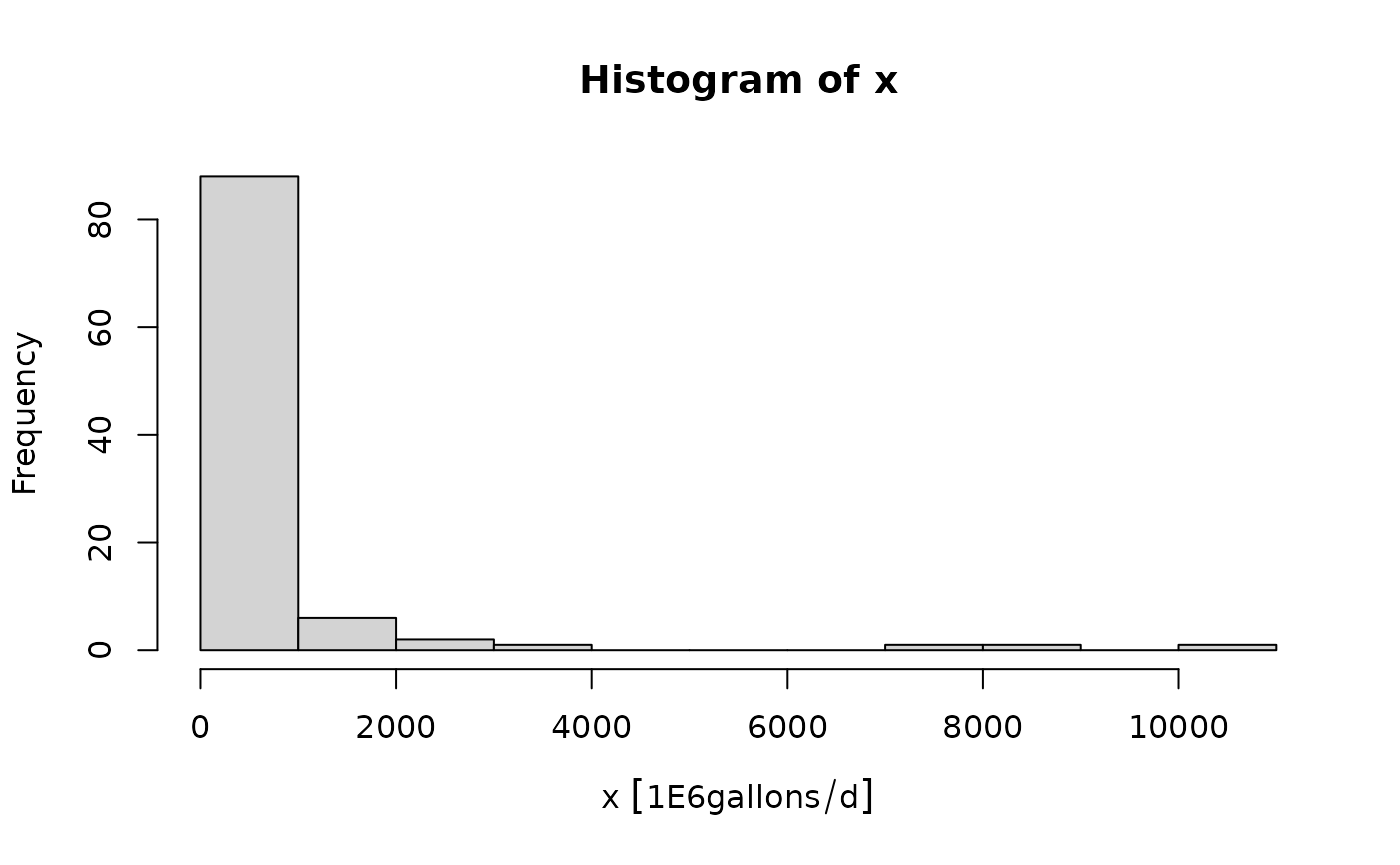
The ggforce package is required to handle plotting units in ggplot2:
library(ggplot2)
library(ggforce)
#> Registered S3 method overwritten by 'ggforce':
#>   method           from
#>   scale_type.units units

ggplot(data.frame(x)) +
geom_histogram(aes(x), binwidth = 100) 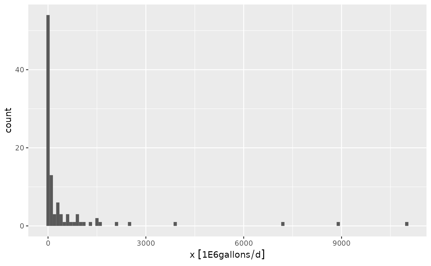
Units with ldc
Stream loads are measured in pounds or kilograms per day for pollutants such as nutrients and sediment. Fecal bacteria loads are typically in colony forming units (cfu) or most probable number (MPN) per day. The included tres_palacios dataset includes bacteria and flow measurements from the Tres Palacios river. Bacteria measurements will need to units in “cfu/100mL” and flow should be in “cubic feet per second.”
library(dplyr)
#>
#> Attaching package: 'dplyr'
#> The following objects are masked from 'package:stats':
#>
#>     filter, lag
#> The following objects are masked from 'package:base':
#>
#>     intersect, setdiff, setequal, union

## create a cfu unit. it is a simple count, so we just add it as an arbitrary unit.
install_unit("cfu")

## format the data for use in ldc
tres_palacios <- as_tibble(tres_palacios) |>
  ## flow must have units, here is is in cfs
  mutate(Flow = set_units(Flow, "ft^3/s"))|>
  ## pollutant concentration must have units
  mutate(Indicator_Bacteria = set_units(Indicator_Bacteria, "cfu/100mL"))
tres_palacios
#> # A tibble: 7,671 × 4
#>    site_no  Date           Flow Indicator_Bacteria
#>    <chr>    <date>     [ft^3/s]        [cfu/100mL]
#>  1 08162600 2000-01-01     0.84                 NA
#>  2 08162600 2000-01-02     3                    NA
#>  3 08162600 2000-01-03     3.4                  NA
#>  4 08162600 2000-01-04     2.6                  NA
#>  5 08162600 2000-01-05     1.6                  NA
#>  6 08162600 2000-01-06     3.2                  NA
#>  7 08162600 2000-01-07    11                    NA
#>  8 08162600 2000-01-08    17                    NA
#>  9 08162600 2000-01-09    22                    NA
#> 10 08162600 2000-01-10    18                    NA
#> # … with 7,661 more rows
The tibble above shows the correct units in each column. What if we want to use metric units for flow?
tres_palacios <- tres_palacios |>
  mutate(Flow = set_units(Flow, "m^3/s"))
tres_palacios
#> # A tibble: 7,671 × 4
#>    site_no  Date          Flow Indicator_Bacteria
#>    <chr>    <date>     [m^3/s]        [cfu/100mL]
#>  1 08162600 2000-01-01  0.0238                 NA
#>  2 08162600 2000-01-02  0.0850                 NA
#>  3 08162600 2000-01-03  0.0963                 NA
#>  4 08162600 2000-01-04  0.0736                 NA
#>  5 08162600 2000-01-05  0.0453                 NA
#>  6 08162600 2000-01-06  0.0906                 NA
#>  7 08162600 2000-01-07  0.311                  NA
#>  8 08162600 2000-01-08  0.481                  NA
#>  9 08162600 2000-01-09  0.623                  NA
#> 10 08162600 2000-01-10  0.510                  NA
#> # … with 7,661 more rows
Now we can calculate the flow and load exceedance probabilities using calc_ldc(). Q and C arguments must have units attached and C must be a concentration unit (mass or counts divided by volume).
## specify the allowable concentration
allowable_concentration <- 126
## set the units
units(allowable_concentration) <- "cfu/100mL"

## calculate the exceedance probabilities along with
## allowable pollutant loads and measured pollutant loads
## at given probabilities
df_ldc <- calc_ldc(tres_palacios,
                   Q = Flow,
                   C = Indicator_Bacteria,
                   allowable_concentration = allowable_concentration)

df_ldc
#> # A tibble: 7,671 × 9
#>    site_no  Date          Flow Indicator_Bacteria Daily_Flow_Volume Daily_Load
#>    <chr>    <date>     [m^3/s]        [cfu/100mL]         [100mL/d]    [cfu/d]
#>  1 08162600 2000-08-18 0.00623                 NA          5382466.         NA
#>  2 08162600 2000-03-07 0.0119                  NA         10275617.         NA
#>  3 08162600 2000-03-06 0.0170                  NA         14679453.         NA
#>  4 08162600 2000-08-22 0.0212                  NA         18349317.         NA
#>  5 08162600 2000-03-08 0.0221                  NA         19083289.         NA
#>  6 08162600 2000-08-17 0.0221                  NA         19083289.         NA
#>  7 08162600 2000-09-11 0.0227                  NA         19572604.         NA
#>  8 08162600 2000-01-01 0.0238                  NA         20551235.         NA
#>  9 08162600 2000-08-21 0.0263                  NA         22753153.         NA
#> 10 08162600 2000-03-05 0.0283                  NA         24465755.         NA
#> # … with 7,661 more rows, and 3 more variables: Allowable_Daily_Load [cfu/d],
#> #   P_Exceedance <dbl>, Flow_Category <fct>
Now we have the percent exceedance for daily flow, flow volume, and allowable daily loads. The daily flow volume and daily load volume are huge numbers, so it might make sense to convert those units.
df_ldc |>
  mutate(Daily_Flow_Volume = set_units(Daily_Flow_Volume, "m^3/day"),
         Allowable_Daily_Load = set_units(Allowable_Daily_Load, "1E9cfu/day"))
#> # A tibble: 7,671 × 9
#>    site_no  Date          Flow Indicator_Bacteria Daily_Flow_Volume Daily_Load
#>    <chr>    <date>     [m^3/s]        [cfu/100mL]           [m^3/d]    [cfu/d]
#>  1 08162600 2000-08-18 0.00623                 NA              538.         NA
#>  2 08162600 2000-03-07 0.0119                  NA             1028.         NA
#>  3 08162600 2000-03-06 0.0170                  NA             1468.         NA
#>  4 08162600 2000-08-22 0.0212                  NA             1835.         NA
#>  5 08162600 2000-03-08 0.0221                  NA             1908.         NA
#>  6 08162600 2000-08-17 0.0221                  NA             1908.         NA
#>  7 08162600 2000-09-11 0.0227                  NA             1957.         NA
#>  8 08162600 2000-01-01 0.0238                  NA             2055.         NA
#>  9 08162600 2000-08-21 0.0263                  NA             2275.         NA
#> 10 08162600 2000-03-05 0.0283                  NA             2447.         NA
#> # … with 7,661 more rows, and 3 more variables:
#> #   Allowable_Daily_Load [1E9cfu/d], P_Exceedance <dbl>, Flow_Category <fct>